Statistics about Linear Regression

Linear regression can build a statistical model which predicts a continuous numerical output using a continuous numerical input(s). Simply, it finds a parameter(s) of a given function \(y=f(x)\) based on \(x\) and \(y\) dataset. The linear regression technique is commonly used in researches to test a theory which describes a relationship between observables. In machine learning courses, the linear regression is probabily what everyone learns in the beginning. It is easy, but very useful.

Let’s learn about background statistical theory about linear regression, and practice with a very fun mini project!

Statistical theory about linear regression

The statistical inference can be categorized into two, the estimation and hypothesis testing. Let’s take a look for the case of linear regression.

Estimation: find the best fitting curve of your dataset

Estimation is infering the true value using the sampled data. Here, you always calculate those two values: the best estimate and the uncertainty of this estimate.

In linear regression, to estimete the parameter of the given function, \(y = wx+b\), the least squares method is used. In the least squares method, the best values of the parameters \(w, b\) make the sum

\[J=\Sigma_{i}^{n}\frac{(y_i-wx_i-b)^2}{\sigma_i^2}\]

minimum, where \(i\) is the index of each data point, \(n\) is the total number of data points, and \(\sigma_i^2\) is an error of variable \(y_i\). The value \(J\) is also called weighted least square.

Dividing an error squere \((y_i-wx_i-b)^2\) by \(\sigma_i^2\) is giving a weight to more precise measurement. In case of a common probability distribution, such as Gaussian (e.g. distribution of heights) or Poisson (e.g. distribution of number of visits for a given visiting probability), the measurement error \(\sigma_i\) is proportional to \(\frac{\sigma}{\sqrt{n}}\), where \(n\) is the number of samples for this measurement and \(\sigma\) is the standard deviation of the theoretical distribution of \(y_i\), which is assumped to be as same as that of the sample.

The \(w, b\) values which minimize the \(J\) satisfies the following equation

\[\nabla{J}=0\]

because the slope of \(J\) is zero at its minimum.

Implementation in machine learning

Linear regression is one of the basic machine learning model. In case of machine learnings, you are using a numerical method to find the parameter values which makes \(\nabla{J}=0\). \(J\) is called the cost function or loss function, and defined as

\[J=\frac{1}{n}\Sigma (y_i-wx_i-b)^2 \text{ like the above, or}\] \[J=\frac{1}{n}\Sigma \|y_i-wx_i-b\| \text{, which is more robust for outliers.}\]

The optimization algorithm to find the minimum \(J\) is called gradient descent. The parameter is updated as

\[w := w-\alpha\nabla{J},\]

where \(\alpha\) is called learning rate, which controls the step size of the paramter updatings. This algorithm makes \(w\) to move in a direction of \(-\nabla{J}=0\), which is a direction of declining \(J\).

Uncertainty of the estimate: goodness of fit

Are you done for linear regression once you found the best line which describe the data? No. For example, you might found the best straight line which minimizes the weighted least square, \(J\), but the data points are acually following a parabola. Then you can’t say you found the best fitting curve. Therefore, once you found the best curve, you should measure the goodness of fit. The goodness of fit is estimated by forming the reduced chi-square,

\[\frac{\chi^2}{\nu}=\frac{J}{\nu}\]

where \(\nu\) is the degree of freedom, equal to the number of data point \(n\) subtracted by the number of parameters (equal to the dimension of the vector \(w\) plus one for \(b\)). Roughly, the smaller the reduced chi-square value, the better the fit is.

Image source: wikipedia

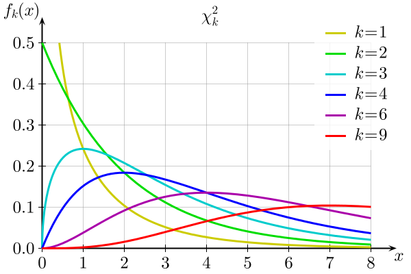
In the figure above, \(k\) is the degree of freedom (like \(\nu\)) and \(f_k(x)\) is the probability density when the \(\chi^2\) is \(x\) for given \(k\). Integrating \(f_k(x)\) gives the probability of getting a \(\chi^2\) value within a certain interval. For example, the probability to get a \(\chi^2\) value larger than 4 when the degree of freedom is 2 is equal to the integration of \(f_2(x)\) from \(x\)=4 to infinite. If this integration is your \(p\)-value, \(x\)=4 is the threshould of your hypothesis test.

Hypothesis test

The probability distribution of \(\chi^2\) depends on \(\nu\), having \(\nu\) as mean and \(2\nu\) as variance. Therefore, \(\frac{\chi^2}{\nu}\) is likely close to 1. Because of this reason, when \(\frac{J}{\nu}\) is close to 1, we say the fit is good, i.e. your linear regression model describes the data points well. If \(\frac{\chi^2}{\nu}\) is much greater than 1, then the data points are not following your model. On the other hand, if \(\frac{\chi^2}{\nu}\) is too smaller than 1, either your model is overfitting your data, or errors of data points are overestimated. Therefore, this reduced chi-square value of linear regression provides a metric of a hypothesis test: if your model follows a certain function or not.