Used Car Acceptance Prediction with Decision Tree

Intro

We will build a decision tree classification model using a used car evaluation dataset.. This is a simple decision tree practice.

Field description

• buying: buying price
• maint: price of the maintenance
• doors: number of doors
• persons: capacity in terms of persons to carry
• lugboot: the size of luggage boot
• safety: estimated safety of the car
• label: unacceptable, acceptable, good, very good

Import packages

from freq_utils import fsize

import numpy as np
import pandas as pd
import matplotlib.pyplot as plt
import seaborn as sns

from sklearn import tree
from sklearn.model_selection import train_test_split
from sklearn.metrics import confusion_matrix
from sklearn.metrics import accuracy_score
from sklearn.metrics import precision_score
from sklearn.metrics import recall_score
from sklearn.metrics import f1_score

Read dataset

df = pd.read_csv("data/car.csv", header=None)

df.info()
df.head()

<class 'pandas.core.frame.DataFrame'>
RangeIndex: 1728 entries, 0 to 1727
Data columns (total 7 columns):
 #   Column  Non-Null Count  Dtype 
---  ------  --------------  ----- 
 0   0       1728 non-null   object
 1   1       1728 non-null   object
 2   2       1728 non-null   object
 3   3       1728 non-null   object
 4   4       1728 non-null   object
 5   5       1728 non-null   object
 6   6       1728 non-null   object
dtypes: object(7)
memory usage: 94.6+ KB

	0	1	2	3	4	5	6
0	vhigh	vhigh	2	2	small	low	unacc
1	vhigh	vhigh	2	2	small	med	unacc
2	vhigh	vhigh	2	2	small	high	unacc
3	vhigh	vhigh	2	2	med	low	unacc
4	vhigh	vhigh	2	2	med	med	unacc

# give them column names
df.columns = ['buying','maint','doors','persons','lugboot','safety','label']

# change data type from object to catetories -- maybe not necessary for this small dataset
df.buying  = pd.Categorical(df.buying, categories=['low', 'med', 'high', 'vhigh'], ordered=True)
df.maint   = pd.Categorical(df.maint, categories=['low', 'med', 'high', 'vhigh'], ordered=True)
df.doors   = pd.Categorical(df.doors, categories=['2', '3', '4', '5more'], ordered=True)
df.persons = pd.Categorical(df.persons, categories=[ '2', '4', 'more'], ordered=True)
df.lugboot = pd.Categorical(df.lugboot, categories=['small', 'med', 'big'], ordered=True)
df.safety  = pd.Categorical(df.safety, categories=['low', 'med', 'high'], ordered=True)
df.label   = pd.Categorical(df.label, categories=['unacc','acc','good','vgood'], ordered=True)

# DecisionTreeClassifier can take only numbers. Let's change type accordingly.
# to binary class
df['class'] = ~(df['label']=='unacc')

# one hot encoding for categorical variables
df = pd.get_dummies(df.iloc[:,0:6]).merge(df,left_index=True,right_index=True)

# check result
print(df.iloc[0])

# check balance
print(df['class'].value_counts())

buying_low           0
buying_med           0
buying_high          0
buying_vhigh         1
maint_low            0
maint_med            0
maint_high           0
maint_vhigh          1
doors_2              1
doors_3              0
doors_4              0
doors_5more          0
persons_2            1
persons_4            0
persons_more         0
lugboot_small        1
lugboot_med          0
lugboot_big          0
safety_low           1
safety_med           0
safety_high          0
buying           vhigh
maint            vhigh
doors                2
persons              2
lugboot          small
safety             low
label            unacc
class            False
Name: 0, dtype: object
False    1210
True      518
Name: class, dtype: int64

More unacceptable cars.

Train test split

# Train test split
train, test = train_test_split(df, train_size = 0.8, test_size = 0.2, random_state=6)

# undersample to make a balanced training set
train = pd.concat([train[train['class']==True], 
                   train[train['class']==False].sample(len(train[train['class']==True]))])

# separate x and y
X_train = train[train.columns[:21]]
X_test = test[test.columns[:21]]
y_train = train['class']
y_test = test['class']

EDA

# select columns to explore
eda = train[['buying','maint','doors','persons','lugboot','safety','label','class']]

Categorical data counts

fsize(16,16)
for i in range(6):
    
    x = eda.columns[i]
    
    #plt.subplot(3,2,i+1)
    sns.catplot(x=x, hue="class", kind="count", data=eda)

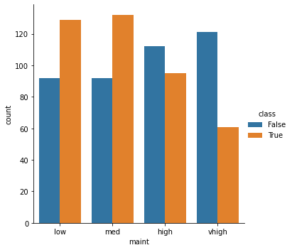
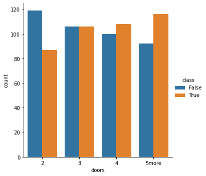
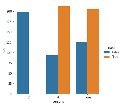
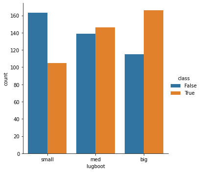
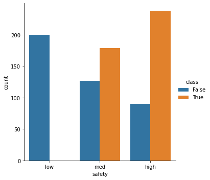
All category have correlation with class. Low “persons” and “safety” have no “acceptable” records.

Feature importance

model = tree.DecisionTreeClassifier(criterion='gini')
model.fit(X_train,y_train)

feature_importances = pd.Series(model.feature_importances_, index=X_train.columns).sort_values(ascending=True)

fsize(10,6)
feature_importances.plot(kind='barh')

<AxesSubplot:>

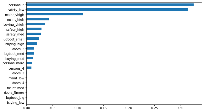
This plot shows one variable correlation with classification. Splitting with person_2 or safety_low makes one purely “unacceptable” node, which explains this high importance.

Train

# fit training set
model = tree.DecisionTreeClassifier(max_depth=7, ccp_alpha=0.01)
model.fit(X_train,y_train) 

# print depth
print('Depth:',model.get_depth())

# plot tree
fsize(12,8)
tree.plot_tree(model, feature_names = X_train.columns, class_names = ['unacc', 'acc'], label='all', filled=True)

Depth: 5





[Text(0.7, 0.9166666666666666, 'safety_low <= 0.5\ngini = 0.5\nsamples = 834\nvalue = [417, 417]\nclass = unacc'),
 Text(0.6, 0.75, 'persons_2 <= 0.5\ngini = 0.45\nsamples = 634\nvalue = [217, 417]\nclass = acc'),
 Text(0.5, 0.5833333333333334, 'buying_vhigh <= 0.5\ngini = 0.294\nsamples = 508\nvalue = [91, 417]\nclass = acc'),
 Text(0.2, 0.4166666666666667, 'buying_high <= 0.5\ngini = 0.212\nsamples = 414\nvalue = [50, 364]\nclass = acc'),
 Text(0.1, 0.25, 'gini = 0.104\nsamples = 292\nvalue = [16, 276]\nclass = acc'),
 Text(0.3, 0.25, 'maint_vhigh <= 0.5\ngini = 0.402\nsamples = 122\nvalue = [34, 88]\nclass = acc'),
 Text(0.2, 0.08333333333333333, 'gini = 0.249\nsamples = 103\nvalue = [15, 88]\nclass = acc'),
 Text(0.4, 0.08333333333333333, 'gini = 0.0\nsamples = 19\nvalue = [19, 0]\nclass = unacc'),
 Text(0.8, 0.4166666666666667, 'maint_high <= 0.5\ngini = 0.492\nsamples = 94\nvalue = [41, 53]\nclass = acc'),
 Text(0.7, 0.25, 'maint_vhigh <= 0.5\ngini = 0.407\nsamples = 74\nvalue = [21, 53]\nclass = acc'),
 Text(0.6, 0.08333333333333333, 'gini = 0.228\nsamples = 61\nvalue = [8, 53]\nclass = acc'),
 Text(0.8, 0.08333333333333333, 'gini = 0.0\nsamples = 13\nvalue = [13, 0]\nclass = unacc'),
 Text(0.9, 0.25, 'gini = 0.0\nsamples = 20\nvalue = [20, 0]\nclass = unacc'),
 Text(0.7, 0.5833333333333334, 'gini = 0.0\nsamples = 126\nvalue = [126, 0]\nclass = unacc'),
 Text(0.8, 0.75, 'gini = 0.0\nsamples = 200\nvalue = [200, 0]\nclass = unacc')]

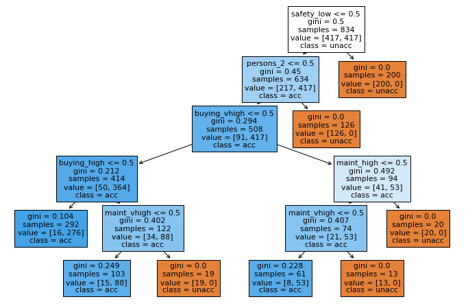
The tree stopped branching before given max_depth. It means the tree is no longer gain information from further splitting. Let’s test the result.

Test

# get prediction
y_pred = model.predict(X_test)

#model.predict_proba(features) # probability
tn, fp, fn, tp = confusion_matrix(y_test, y_pred).ravel()
print(tn, fp, fn, tp)

# Score
print('Scores')
#print(model.score(X_test, y_test)) # accuracy
print('Accuracy:',accuracy_score(y_test, y_pred))
print('Precision:',precision_score(y_test, y_pred))
print('Recall:',recall_score(y_test, y_pred))
print('F1:',f1_score(y_test, y_pred))

# plot distributions for leading two features
test['pred']= y_pred

232 13 0 101
Scores
Accuracy: 0.9624277456647399
Precision: 0.8859649122807017
Recall: 1.0
F1: 0.9395348837209303