Housing price prediction with linear regression

May 1, 2022

Intro

This project is the famous housing price prediction. Description of data field can be found at the dataset source.

Overview

Here, I’ll show

EDA of numerical and categorical features with visualization
Feature engineering (some of them are not existing method, as far as I know)
- Change categorical feature into numerical feature
- Impute empty entry in a way less impact on linear regression
- Feature selection
- Cleaning
Training
- Hyperparameter tuning
  - Regularization and learning rate tuning with ElasticNet
  - Tune feature selection
Test result
- Visualize the fitting result and residuals
- List important features
Conclusion
- Show how precise this model is for a practical metric for potential users.

Load dataset

# import modules
import numpy as np
import pandas as pd
import matplotlib.pyplot as plt
import seaborn as sns

#import statsmodels.formula.api as smf

#from sklearn.decomposition import PCA # tested and didn't help
from sklearn.model_selection import train_test_split, cross_val_score
from sklearn.linear_model import LinearRegression, ElasticNetCV
from sklearn.model_selection import learning_curve
from sklearn.model_selection import ShuffleSplit
from sklearn.preprocessing import StandardScaler
import sklearn.metrics as metrics

# figure cosmetic function
def fsize(w,h,c=False):
    
    # set figure size
    plt.rcParams["figure.figsize"] = [w, h]
    
    # adjust plot automatically
    plt.rcParams['figure.constrained_layout.use'] = c

# import training data
df = pd.read_csv("data/house.csv")
df_sub = pd.read_csv("data/house_test.csv")

df.info()
df.head(5)

# check duplicated entries
print(df.duplicated().value_counts())
print(df_sub.duplicated().value_counts())

<class 'pandas.core.frame.DataFrame'>
RangeIndex: 1460 entries, 0 to 1459
Data columns (total 81 columns):
 #   Column         Non-Null Count  Dtype  
---  ------         --------------  -----  
 Id             1460 non-null   int64  
 MSSubClass     1460 non-null   int64  
 MSZoning       1460 non-null   object 
 LotFrontage    1201 non-null   float64
 LotArea        1460 non-null   int64  
 Street         1460 non-null   object 
 Alley          91 non-null     object 
 LotShape       1460 non-null   object 
 LandContour    1460 non-null   object 
 Utilities      1460 non-null   object 
LotConfig      1460 non-null   object 
LandSlope      1460 non-null   object 
Neighborhood   1460 non-null   object 
Condition1     1460 non-null   object 
Condition2     1460 non-null   object 
BldgType       1460 non-null   object 
HouseStyle     1460 non-null   object 
OverallQual    1460 non-null   int64  
OverallCond    1460 non-null   int64  
YearBuilt      1460 non-null   int64  
YearRemodAdd   1460 non-null   int64  
RoofStyle      1460 non-null   object 
RoofMatl       1460 non-null   object 
Exterior1st    1460 non-null   object 
Exterior2nd    1460 non-null   object 
MasVnrType     1452 non-null   object 
MasVnrArea     1452 non-null   float64
ExterQual      1460 non-null   object 
ExterCond      1460 non-null   object 
Foundation     1460 non-null   object 
BsmtQual       1423 non-null   object 
BsmtCond       1423 non-null   object 
BsmtExposure   1422 non-null   object 
BsmtFinType1   1423 non-null   object 
BsmtFinSF1     1460 non-null   int64  
BsmtFinType2   1422 non-null   object 
BsmtFinSF2     1460 non-null   int64  
BsmtUnfSF      1460 non-null   int64  
TotalBsmtSF    1460 non-null   int64  
Heating        1460 non-null   object 
HeatingQC      1460 non-null   object 
CentralAir     1460 non-null   object 
Electrical     1459 non-null   object 
1stFlrSF       1460 non-null   int64  
2ndFlrSF       1460 non-null   int64  
LowQualFinSF   1460 non-null   int64  
GrLivArea      1460 non-null   int64  
BsmtFullBath   1460 non-null   int64  
BsmtHalfBath   1460 non-null   int64  
FullBath       1460 non-null   int64  
HalfBath       1460 non-null   int64  
BedroomAbvGr   1460 non-null   int64  
KitchenAbvGr   1460 non-null   int64  
KitchenQual    1460 non-null   object 
TotRmsAbvGrd   1460 non-null   int64  
Functional     1460 non-null   object 
Fireplaces     1460 non-null   int64  
FireplaceQu    770 non-null    object 
GarageType     1379 non-null   object 
GarageYrBlt    1379 non-null   float64
GarageFinish   1379 non-null   object 
GarageCars     1460 non-null   int64  
GarageArea     1460 non-null   int64  
GarageQual     1379 non-null   object 
GarageCond     1379 non-null   object 
PavedDrive     1460 non-null   object 
WoodDeckSF     1460 non-null   int64  
OpenPorchSF    1460 non-null   int64  
EnclosedPorch  1460 non-null   int64  
3SsnPorch      1460 non-null   int64  
ScreenPorch    1460 non-null   int64  
PoolArea       1460 non-null   int64  
PoolQC         7 non-null      object 
Fence          281 non-null    object 
MiscFeature    54 non-null     object 
MiscVal        1460 non-null   int64  
MoSold         1460 non-null   int64  
YrSold         1460 non-null   int64  
SaleType       1460 non-null   object 
SaleCondition  1460 non-null   object 
SalePrice      1460 non-null   int64  
dtypes: float64(3), int64(35), object(43)
memory usage: 924.0+ KB
False    1460
dtype: int64
False    1459
dtype: int64

# rename columns to follow variable naming for convenience
df.rename(columns={'1stFlrSF':'FlrSF1st', '2ndFlrSF':'FlrSF2nd', '3SsnPorch':'Porch3Ssn'}, inplace=True) 
df_sub.rename(columns={'1stFlrSF':'FlrSF1st', '2ndFlrSF':'FlrSF2nd', '3SsnPorch':'Porch3Ssn'}, inplace=True) 

Split train/dev/test set before exploration

Test set will be used only for testing purpose. Shouldn’t be used for exploration and feature engineering.

df, df_test = train_test_split(df, test_size=0.2, random_state=20)

EDA with Feature Engineering

Check price distribution and make it log scale

# plot
fsize(8,5)
ax = plt.hist(df.SalePrice,bins=30)

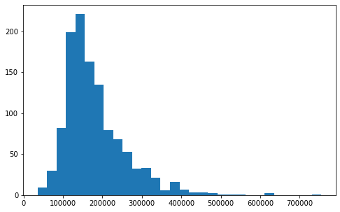
Distribution is skewed. Let’s even out for better linear regression performance.

# Change to log scale
df.SalePrice = np.log10(df.SalePrice) # train set
df_test.SalePrice = np.log10(df_test.SalePrice) # test set

# plot result
ax = plt.hist(df.SalePrice,bins=30)

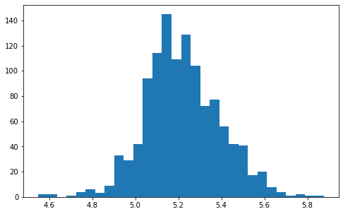
Now close to normal distribution.

Check numerical feature distirubution and clean them a bit

#%%script false --no-raise-error

# get a list of numerical features
features = df.dtypes[df.dtypes!='object'].index.tolist()

# drop the target column
features = features[:-1] 
n = len(features)

# set figure size
fsize(16,n,True)

# plot histograms
for i in range(n):
             
    plt.subplot(n//4+n%4, 4, i+1)

    plt.hist(df[features[i]],bins=30)
    plt.title(features[i])
    plt.xlabel(features[i])

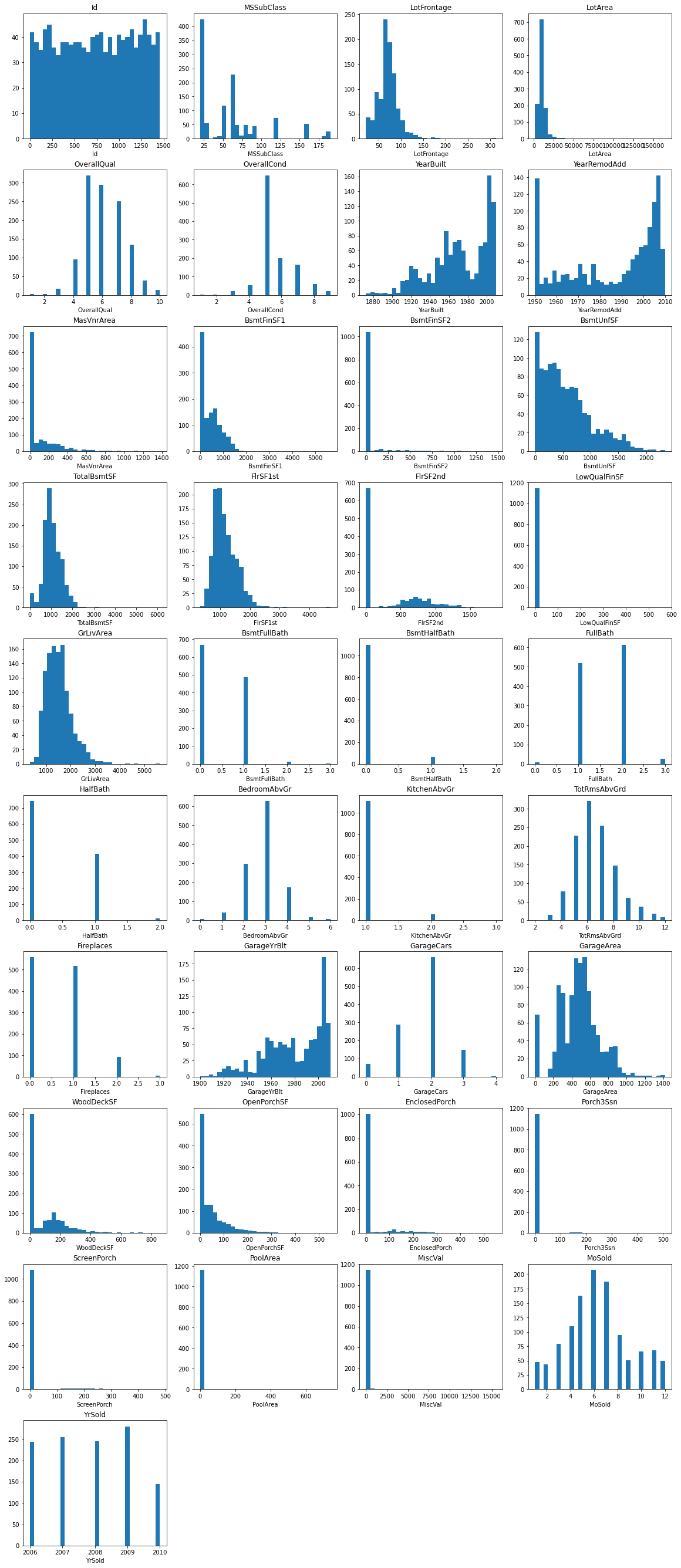
A little cleaning

# skewed features (we will use these lists soon)
left_skewed = ['LotFrontage','LotArea','MasVnrArea',
               'BsmtFinSF1','BsmtFinSF2','BsmtUnfSF','TotalBsmtSF',
               'FlrSF1st','FlrSF2nd','GrLivArea',
               'GarageArea','WoodDeckSF','OpenPorchSF','EnclosedPorch',
               'MiscVal','SalePrice'] # all sizes, makes sense
right_skewed = ['YearBuilt','YearRemodAdd','GarageYrBlt'] # all years, makes sense      

# drop redundunt feature
df.drop(['Id'],axis=1,inplace=True) # train set
df_test.drop(['Id'],axis=1,inplace=True) # test

# this feature should be categorical
df = df.astype({'MSSubClass':str})
df_test = df_test.astype({'MSSubClass':str})
df_sub = df_sub.astype({'MSSubClass':str})

Impute numerical feature

Non of valid numerical feature has zero value. Set empty entry as zero for now. Meaning of empty entry is this house doesn’t have corresponding material/place, i.e. N/A.

# get a list of numerical features after cleaning
features = df.dtypes[df.dtypes!='object'].index.tolist()
# drop the target column
features = features[:-1] 

# impute empty value with 0
# I'll handle imputation later soon

for x in features:
    
    df.fillna({x: 0},inplace=True) 
    df_test.fillna({x: 0},inplace=True)
    df_sub.fillna({x: 0},inplace=True)

    #avg = df[x].mean()

    #df.fillna({x: avg},inplace=True) 
    #df_test.fillna({x: avg},inplace=True) 

Check categorical feature distirubution and clean/impute them

#%%script false --no-raise-error

# get a list of categorical features
features = df.dtypes[df.dtypes=='object'].index.tolist()

n = len(features)

# set figure size
fsize(16,2*n,True)

# plot histograms
for i in range(n):
             
    plt.subplot(n//2+n%2, 2, i+1)

    sns.boxplot(x=features[i], y="SalePrice", data=df)
    sns.stripplot(x=features[i], y="SalePrice", data=df, alpha=0.3)
    plt.title(features[i])
    plt.xlabel(features[i])

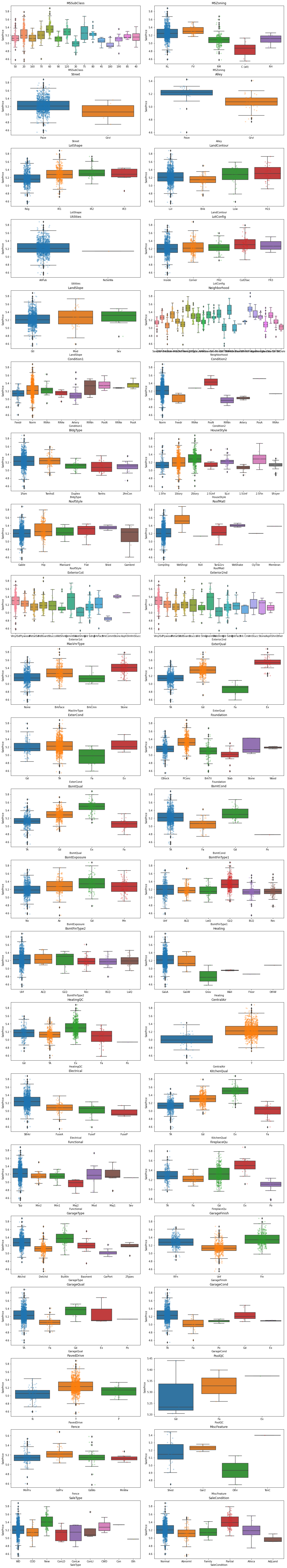
A little cleaning and imputation

# impute empty data - empty for unknown reason
df.fillna({'MasVnrType':'Unknown'},inplace=True)
df.fillna({'Electrical':'Unknown'},inplace=True)

df_test.fillna({'MasVnrType':'Unknown'},inplace=True)
df_test.fillna({'Electrical':'Unknown'},inplace=True)

df_sub.fillna({'MasVnrType':'Unknown'},inplace=True)
df_sub.fillna({'Electrical':'Unknown'},inplace=True)

# get a list of categorical features
features = df.dtypes[df.dtypes=='object'].index.tolist()

# impute empty data - when a house doesn't have this material
for x in features:
    df.fillna({x: 'NotUsed'},inplace=True) 
    df_test.fillna({x: 'NotUsed'},inplace=True) 
    df_sub.fillna({x: 'NotUsed'},inplace=True) 

Change categorical features to numerical features

Here, I’ll make a categorical feature into numeric ones, then perform linear regression. For each feature, they way how I transform is

calculate mean value of SalePrice for each category
replace the category by the mean SalePrice value

# get a list of categorical features
features = df.dtypes[df.dtypes=='object'].index.tolist()

# Get avarage to fill rare entry
avg = df.SalePrice.mean()

for x in features:
    
    # make a dictionary of {category: mean of SalePrice of that category}
    # use only train set
    dic = df.groupby([x]).SalePrice.mean().to_dict()
       
    # Change categorical value into average sale price
    # fill dev and test set values by values obtained from train set
    def cat_to_num(x):
        try:
            return dic[x]
        except:
            # exception when the rare category is not shown in training set
            return avg
    
    
    df[x] = df[x].apply(lambda x: cat_to_num(x))
    df_test[x] = df_test[x].apply(lambda x: cat_to_num(x))
    df_sub[x] = df_sub[x].apply(lambda x: cat_to_num(x))

# for nan entries of rare categories
# fill average of training set
for x in df_test.columns[:-1]:
    df_test[x].fillna(df[x].mean(), inplace=True)

for x in df_sub.columns[1:]:
    df_sub[x].fillna(df[x].mean(), inplace=True)

# check result
df.head(5)

# we shouldn't have nan now.
df.isna().value_counts()

MSSubClass  MSZoning  LotFrontage  LotArea  Street  Alley  LotShape  LandContour  Utilities  LotConfig  LandSlope  Neighborhood  Condition1  Condition2  BldgType  HouseStyle  OverallQual  OverallCond  YearBuilt  YearRemodAdd  RoofStyle  RoofMatl  Exterior1st  Exterior2nd  MasVnrType  MasVnrArea  ExterQual  ExterCond  Foundation  BsmtQual  BsmtCond  BsmtExposure  BsmtFinType1  BsmtFinSF1  BsmtFinType2  BsmtFinSF2  BsmtUnfSF  TotalBsmtSF  Heating  HeatingQC  CentralAir  Electrical  FlrSF1st  FlrSF2nd  LowQualFinSF  GrLivArea  BsmtFullBath  BsmtHalfBath  FullBath  HalfBath  BedroomAbvGr  KitchenAbvGr  KitchenQual  TotRmsAbvGrd  Functional  Fireplaces  FireplaceQu  GarageType  GarageYrBlt  GarageFinish  GarageCars  GarageArea  GarageQual  GarageCond  PavedDrive  WoodDeckSF  OpenPorchSF  EnclosedPorch  Porch3Ssn  ScreenPorch  PoolArea  PoolQC  Fence  MiscFeature  MiscVal  MoSold  YrSold  SaleType  SaleCondition  SalePrice
False       False     False        False    False   False  False     False        False      False      False      False         False       False       False     False       False        False        False      False         False      False     False        False        False       False       False      False      False       False     False     False         False         False       False         False       False      False        False    False      False       False       False     False     False         False      False         False         False     False     False         False         False        False         False       False       False        False       False        False         False       False       False       False       False       False       False        False          False      False        False     False   False  False        False    False   False   False     False          False        1168
dtype: int64

Numerical feature imputation and scaling for linear regression

For numerical features, 0 value means eigher there’s no such material or data is empty. Here, I made an imputation technique, which fill the empty record by

1. perform linear regressionn with filled records ($y = mx + b$)
1. get the average SalePrice of empty record ($=y0$)
1. calculate the corresponding x value of y0 on the linear regression curve found at step 1 ($x0 = (y0-b)/m$)
1. impute empty record with $x0$

Numerical feature imputation

def get_scaling_parameter(df):
    
    # feature scaling function
    def feature_scaling(df, x):
    
        mu = np.mean(df[x])
        sig = np.std(df[x])
    
        return mu, sig
    
    # features need singular dat atransform
    lst_return =[]

    for i in range(len(df.columns)-1):
        
        x = df.columns[i]
          
        regular  = df.loc[df[x]!=0, [x,'SalePrice']].copy()
        singular = df.loc[df[x]==0, [x,'SalePrice']].copy()
        
        if x in left_skewed:
            regular[x]  = np.log10(regular[x]+1)
            singular[x] = np.log10(singular[x]+1)
        
        if x in right_skewed:
            regular[x]  = np.log10(2030-regular[x])
            singular[x] = np.log10(2030-singular[x])
        

        mu, sig = feature_scaling(regular, x)
            
        #regular[x] = (regular[x]-mu)/sig
            
        #results = smf.ols('SalePrice'+'~'+x, data=regular).fit()
        #b, m = results.params
        #b_err, m_err = results.bse
        
        model = LinearRegression()
        model.fit(regular[x].to_numpy().reshape(-1,1),regular.SalePrice.to_numpy())
        
        b = model.intercept_
        m = model.coef_.squeeze()
                
        singular_y_mean = np.mean(singular['SalePrice']) 
        singular_x_shift = (singular_y_mean-b)/m
        
        lst_return.append([x,mu,sig,singular_x_shift])
            
    return lst_return

def sdp_transform(df, lst_scale_par):
    
    df_copy = df.copy()

    for item in lst_scale_par:
        
        x, mu, sig, shift = item
     
        if np.isnan(mu): 
            print('err')
            df_copy.drop([x], axis=1, inplace=True)

        else:
            
            regular  = df.loc[df[x]!=0, [x]].copy()
            singular = df.loc[df[x]==0, [x]].copy()
            
            if x in left_skewed:
                regular[x]  = np.log10(regular[x]+1)
                #singular[x] = np.log10(singular[x]+1)
        
            if x in right_skewed:
                regular[x]  = np.log10(2030-regular[x])
                #singular[x] = np.log10(2030-singular[x])
 
            #regular[x] = (regular[x]-mu)/sig
            singular[x] = shift
            
            df_add = regular[[x]]
                        
            if len(singular)>0 :
                df_add = pd.concat([df_add, singular[[x]]])
                
            df_copy[x] = df_add[x]

    return df_copy

lst_scale_par = get_scaling_parameter(df)


df = sdp_transform(df,lst_scale_par)
df_test = sdp_transform(df_test,lst_scale_par)
df_sub = sdp_transform(df_sub,lst_scale_par)

/Users/minjungkim/opt/anaconda3/lib/python3.8/site-packages/pandas/core/arraylike.py:397: RuntimeWarning: invalid value encountered in log10
  result = getattr(ufunc, method)(*inputs, **kwargs)

“RuntimeWarning: invalid value encountered in log10” is from a few NaN entries of rare categories. It will be handled later.

Feature scaling

Feature scaling improves optimization performance and give a fair weight to each feature. Here, I’m using standardization, which is more robust to outliers compared to min-max normalization. $x_{j} \rightarrow \frac{x_{j}-\mu_{j}}{\sigma_{j}},$ where $x$ is data value, $j$ is feature index, $\mu_{j}$ is mean of $x_{J}$, and $\sigma_{j}$ is standard deviation of $x_{J}$.

scaler = StandardScaler()

# fit with training set
scaler.fit(df.drop('SalePrice',axis=1))

# transform all sets
df[df.columns[:-1]] = scaler.transform(df.drop('SalePrice',axis=1))
df_test[df_test.columns[:-1]] = scaler.transform(df_test.drop('SalePrice',axis=1))
df_sub[df_sub.columns[1:]] = scaler.transform(df_sub.drop('Id',axis=1))

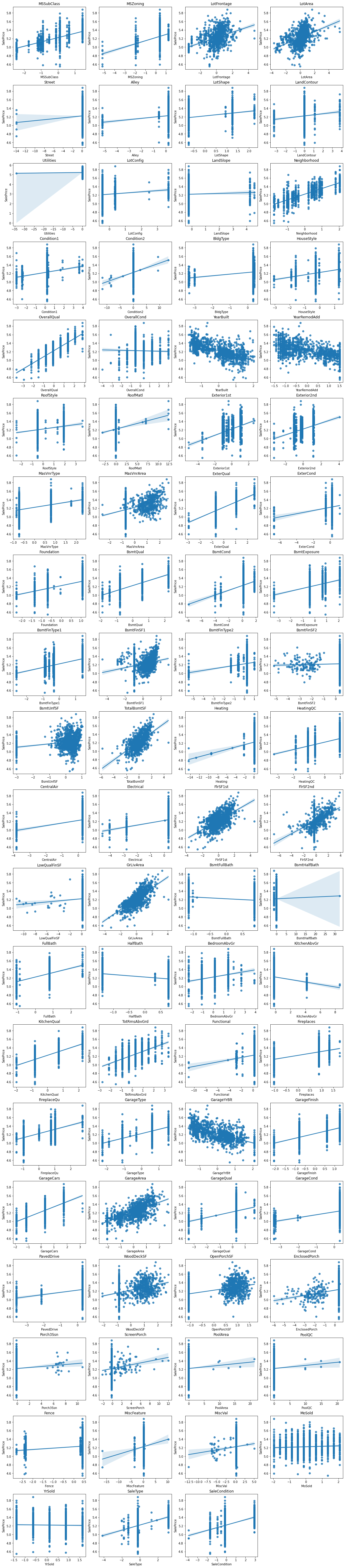
SalePrice vs Feature

#%%script false --no-raise-error

# Plot one variable linear regression of each feature
# x: feature, y: SalePrice

n = len(df.columns)-1
fsize(16,n,True)

for i in range(n):
    
    x=df.columns[i]
    
    plt.subplot(n//4+n%4,4,i+1)
    sns.regplot(x=x, y='SalePrice', data=df)
    plt.title(x)

Select input features

Sort features in an order of correlation with SalePrice, then remove highly correlated features with them.

def select_feature(threshold0=0.5, threshold1=0.6):

    # Select features highly correlated with SalePrice
    features = df.corr().SalePrice.apply(lambda x: abs(x)).sort_values(ascending=False)
    high_corr_features = features[features>threshold0].drop('SalePrice')
    

    # Select highly correlating columns
    columns_to_drop = []
    for x in high_corr_features.index:

        if x in columns_to_drop:
            continue

        for y in high_corr_features.index:

            if x==y:
                continue
            val = df[x].corr(df[y])
            if val>threshold1:
                columns_to_drop.append(y)
                
    
    corr_features = [x for x in high_corr_features.index if not x in columns_to_drop]
    return corr_features


corr_features = select_feature(0.6, 0.6)
corr_features

['OverallQual', 'GarageArea', 'YearBuilt', 'GarageFinish', 'TotalBsmtSF']

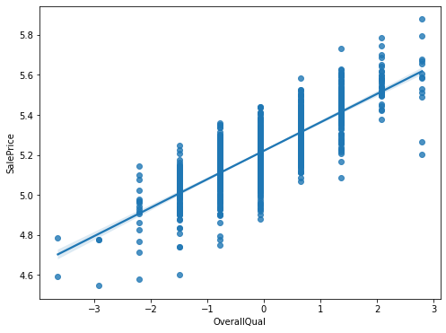
# Plot one highly correlating example
fsize(8,6)
sns.regplot(x='OverallQual', y='SalePrice', data=df)

<AxesSubplot:xlabel='OverallQual', ylabel='SalePrice'>

Train

I’m using root mean squared error (RMSE) as the scoring metric. When I calculate RMSE, the SalePrice is log transformed.

# Make a scorer
def cost_function(y, y_pred):
    
    # flip sign for make_scorer function to give positive output
    return -1.0*(np.square(y_pred-y).sum()/len(y))**0.5

scorer = metrics.make_scorer(cost_function, greater_is_better=False)

Plot learning curve

Plot learning curve to check sign of overfitting.

X_train = df[corr_features]
y_train = df.SalePrice

def plot_learning_curve(estimator, title, X, y, scoring=None, ylim=None, cv=None,
                        train_sizes=np.linspace(.1, 1.0, 5)):

    # Copied and modified scikit-learn document
    ax = plt.subplot()

    ax.set_title(title)
    if ylim is not None:
        ax.set_ylim(*ylim)
    ax.set_xlabel("Training examples size")
    ax.set_ylabel("std of difference in percents")

    train_sizes, train_scores, test_scores = \
        learning_curve(estimator, X, y, scoring=scoring, cv=cv, train_sizes=train_sizes)
    
    train_scores_mean = np.mean(train_scores, axis=1)
    train_scores_std = np.std(train_scores, axis=1)
    test_scores_mean = np.mean(test_scores, axis=1)
    test_scores_std = np.std(test_scores, axis=1)

    # Plot learning curve
    ax.grid()
    ax.fill_between(train_sizes, train_scores_mean - train_scores_std,
                         train_scores_mean + train_scores_std, alpha=0.1,
                         color="r")
    ax.fill_between(train_sizes, test_scores_mean - test_scores_std,
                         test_scores_mean + test_scores_std, alpha=0.1,
                         color="g")
    ax.plot(train_sizes, train_scores_mean, 'o-', color="r",
                 label="Training score")
    ax.plot(train_sizes, test_scores_mean, 'o-', color="g",
                 label="Cross-validation score")
    ax.legend(loc="best")

    return plt

def learning_curve_wrapper(X,y):
    
    n_samples = X.shape[0]
    cv = ShuffleSplit(n_splits=5, test_size=0.3, random_state=0)

    model = LinearRegression()
    scorer = metrics.make_scorer(cost_function, greater_is_better=False)

    title = "Learning Curves"

    plot_learning_curve(model, title, X, y, scoring=scorer, train_sizes=np.linspace(.1, 1.0, 20))


    plt.show()
    
    return model

    
model = learning_curve_wrapper(X_train, y_train)

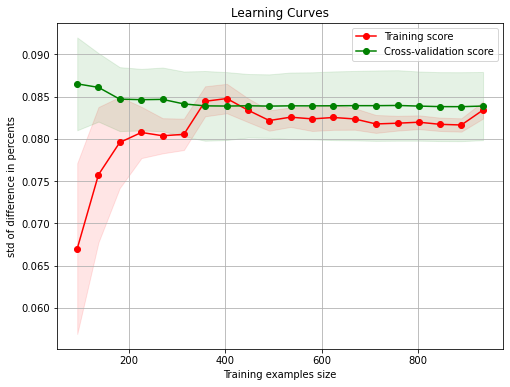
Both training and validation set are converging at quite low error. Good!

Hyperparameter tuning

Select features
Optimize ElasticNet regularization parameters and learning rate

# define a function to tune regularization and learning rate
# linear regression with ElasticNet
def tuneElasticNet(X_train,y_train):
    
    # 1st iteration to find scale
    model = ElasticNetCV(l1_ratio = [0.001, 0.003, 0.01, 0.03, 0.1, 0.3, 0.6, 1],
                              alphas = [0.0001, 0.0003, 0.0006, 0.001, 0.003, 0.006, 
                                        0.01, 0.03, 0.06, 0.1, 0.3, 0.6, 1, 3, 6], 
                              max_iter = 10000, cv = 10, n_jobs=-1,
                              fit_intercept=True)

    model.fit(X_train, y_train)
    if (model.l1_ratio_ > 1):
        model.l1_ratio_ = 1    
        
    alpha = model.alpha_
    l1_ratio = model.l1_ratio_
    #print("1st iteration - l1_ratio, alpha :", ratio, alpha)


    # 2nd iteration for fine tuning
    
    l1_ratio_temp = [l1_ratio*0.5, l1_ratio*0.8, l1_ratio, l1_ratio*1.2, l1_ratio*1.5]
    
    
    model = ElasticNetCV(l1_ratio = [x if x<=1 else 1 for x in l1_ratio_temp ],
                              alphas = [alpha*0.1 , alpha*0.3, alpha, alpha*3, alpha*10], 
                              max_iter = 10000, cv = 5, n_jobs=-1,
                              fit_intercept=True)

    model.fit(X_train, y_train)
    if (model.l1_ratio_ > 1):
        model.l1_ratio_ = 1    

    alpha = model.alpha_
    l1_ratio = model.l1_ratio_
    #print("2nd iteration - l1_ratio, alpha :", ratio, alpha)


    # 3rd iteration for fine tuning
    
    l1_ratio_temp = [l1_ratio*0.8, l1_ratio*0.85, l1_ratio*0.9, l1_ratio*0.95, l1_ratio,
                     l1_ratio*1.05, l1_ratio*1.1, l1_ratio*1.15, l1_ratio*1.2]

    model = ElasticNetCV(l1_ratio = [x if x<=1 else 1 for x in l1_ratio_temp ],
                              alphas = [alpha*0.8, alpha*0.9, alpha, alpha*1.1, alpha*1.2], 
                              max_iter = 10000, cv = 5, n_jobs=-1,
                              fit_intercept=True)

    model.fit(X_train, y_train)
    if (model.l1_ratio_ > 1):
        model.l1_ratio_ = 1    
        
        
    alpha = model.alpha_
    l1_ratio = model.l1_ratio_
    #print("3rd iteration - l1_ratio, alpha :", ratio, alpha)

    # Cross validation score
    #print("Score:", cross_val_score(model, X_train, y_train, cv=5, scoring=scorer).mean())    
    
    return model, cross_val_score(model, X_train, y_train, cv=5, scoring=scorer).mean()

# Train and Hyperparameter tuning -- 1st iteration

params = []

# found out ranges through iterations
for th0 in (0, 0.1, 0.2): 
        #(0.1, 0.2, 0.3, 0.4, 0.5, 0.6, 0.7, 0.8):
    for th1 in (0.7, 0.8):
        #(0.1, 0.2, 0.3, 0.4, 0.5, 0.6, 0.7, 0.8):
        
        corr_features = select_feature(th0, th1)

        X_train = df[corr_features]
        y_train = df.SalePrice
        
        model, score = tuneElasticNet(X_train,y_train)
        
        params.append((model,th0,th1,score))

def takeFourth(elem):
    return elem[3]

params.sort(key=takeFourth)
[params[i][1:] for i in range(0,5)]

[(0, 0.8, 0.054934925785856605),
 (0, 0.7, 0.055045021987165335),
 (0.1, 0.8, 0.05660590767588628),
 (0.1, 0.7, 0.05667749672828577),
 (0.2, 0.7, 0.058364893449542175)]

Threshold0 = 0 and Threshold1 = 0.7-0.8 gave the least error, 0.055. Overall, the sorted result indicate that taking all parameters gives the best result with regularization.

Test and Residual Analysis

# final model
model, th0, th1, score = params[0]
corr_features = select_feature(th0, th1)

# test set
X_test = df_test[corr_features]
y_test = df_test.SalePrice

# check nan entry
X_test[X_test.isna().any(axis=1)]

	OverallQual	Neighborhood	GrLivArea	ExterQual	KitchenQual	GarageCars	BsmtQual	YearBuilt	GarageFinish	TotalBsmtSF	...	Porch3Ssn	Street	MoSold	LandSlope	PoolArea	BsmtFinSF2	YrSold	OverallCond	Utilities	BsmtHalfBath
954	-0.064865	-1.020837	-1.126258	-0.68169	-0.80258	-1.898184	0.600439	0.125701	-2.090759	-0.137196	...	-0.13691	0.071858	1.34402	-0.232617	-0.067759	0.343611	-1.392892	-0.510559	0.029273	32.454951

1 rows × 71 columns

# there's just a nan entry
# let's fill with average

for x in X_test.columns:
    X_test[x].fillna(X_test[x].mean(), inplace=True)

/var/folders/31/7v9nfdf14sz0sxn2xwnq90y00000gn/T/ipykernel_94749/8326161.py:5: SettingWithCopyWarning: 
A value is trying to be set on a copy of a slice from a DataFrame

See the caveats in the documentation: https://pandas.pydata.org/pandas-docs/stable/user_guide/indexing.html#returning-a-view-versus-a-copy
  X_test[x].fillna(X_test[x].mean(), inplace=True)

# predict
y_pred = model.predict(X_test)

fsize(8,6)

# Plot predictions
plt.scatter(y_test, y_pred)
plt.title("Prediction")
plt.ylabel("Predicted price")
plt.xlabel("Real price")
plt.plot([4.5, 6], [4.5,6], c = "red")
plt.show()

print('R^2 of y_pred and y_test:',model.score(X_test,y_test))


# Plot residue
residuals = y_pred - y_test
plt.scatter(y_pred, residuals, alpha=0.4)
plt.title('Residue')
plt.xlabel("Predicted price")
plt.hlines(y = 0, xmin = 4.8, xmax = 5.7, color = "red")
plt.show()

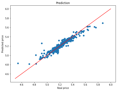
R^2 of y_pred and y_test: 0.9025793776944269

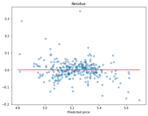
A little deviations at very low or high prices. Otherwise, good.

# Plot features with high coefficient (leading features)
coefs = pd.Series(model.coef_, index = corr_features)

coefs = pd.concat([coefs.sort_values().head(7),
                     coefs.sort_values().tail(8)])
coefs.plot.barh()
ax = plt.title("Coefficients of used features")

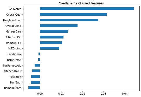
So, good to have large great room and overall high quality/condition with large garage in expensive neighbor. Having a basement is good, but it better not have a bathroom.

Conclusion

What should be the final metric? I think the most important metric for users will be how precisely we predict the house price in percent.

# so far, we've used log scale price
# now, conver to real value
y_pred = 10**y_pred
y_test = 10**y_test

# difference in percent
y_diff = (y_pred-y_test)/y_test

plt.hist(y_diff, bins=30)

total_count = len(y_diff)

precise_count = len(y_diff[y_diff<0.2])
print('Predict housing price within 20% for ',precise_count/total_count*100,'% of data') 

precise_count = len(y_diff[y_diff<0.1])
print('Predict housing price within 10% for ',precise_count/total_count*100,'% of data')

Predict housing price within 20% for  95.2054794520548 % of data
Predict housing price within 10% for  86.64383561643835 % of data

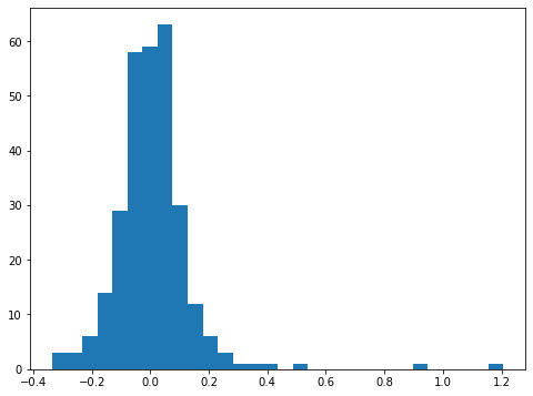
Would you buy this model? I would definetly.

Submission to Kaggle

# test set
X_sub = df_sub[['Id']+corr_features]

# check nan entry
X_sub[X_sub.isna().any(axis=1)]

	Id	OverallQual	Neighborhood	GrLivArea	ExterQual	KitchenQual	GarageCars	BsmtQual	YearBuilt	GarageFinish	...	Porch3Ssn	Street	MoSold	LandSlope	PoolArea	BsmtFinSF2	YrSold	OverallCond	Utilities	BsmtHalfBath
1127	2588	0.649874	-0.363391	-1.320127	-0.68169	-0.80258	-1.151364	-0.785915	0.125701	-0.797912	...	-0.13691	0.071858	-1.233069	-0.232617	-0.067759	-2.069423	-0.640047	0.367693	0.029273	-1.313451
1399	2860	-0.064865	-1.020837	-1.030939	-0.68169	-0.80258	-1.898184	0.600439	0.125701	-2.090759	...	-0.13691	0.071858	1.344020	-0.232617	-0.067759	0.343611	-1.392892	-0.510559	0.029273	32.454951

2 rows × 72 columns

# there's just two nan entry
# let's fill with average

for x in X_sub.columns:
    X_sub[x].fillna(X_sub[x].mean(), inplace=True)

/var/folders/31/7v9nfdf14sz0sxn2xwnq90y00000gn/T/ipykernel_94749/172487346.py:5: SettingWithCopyWarning: 
A value is trying to be set on a copy of a slice from a DataFrame

See the caveats in the documentation: https://pandas.pydata.org/pandas-docs/stable/user_guide/indexing.html#returning-a-view-versus-a-copy
  X_sub[x].fillna(X_sub[x].mean(), inplace=True)

# predict
y_pred = model.predict(X_sub.drop('Id',axis=1))
y_pred = 10**y_pred

# make a submission format
X_sub['SalePrice'] = y_pred

submit = X_sub[['Id','SalePrice']]

# save
submit.to_csv('data/house_submission.csv',index=False)

/var/folders/31/7v9nfdf14sz0sxn2xwnq90y00000gn/T/ipykernel_94749/1023321855.py:2: SettingWithCopyWarning: 
A value is trying to be set on a copy of a slice from a DataFrame.
Try using .loc[row_indexer,col_indexer] = value instead

See the caveats in the documentation: https://pandas.pydata.org/pandas-docs/stable/user_guide/indexing.html#returning-a-view-versus-a-copy
  X_sub['SalePrice'] = y_pred

Done.

Share on

Twitter Facebook LinkedIn