Credit Card Fraud Detection with Logistic Regression

Intro

We will build a logistic regression model using PCA transformed data. Dataset: data/creditcard.csv source: Kaggle

The assumption of this model is that both of normal and fraud transactions can be separated by a single linear boundary. Also, I assumed the fraud techniques stay same, i.e. this model is valid over long term (otherwise, this model becomes useless other than self practice purpose).

Import packages

from freq_utils import fsize, plot_learning_curve # freq_utils.py is my custom file

import numpy as np
import pandas as pd
import matplotlib.pyplot as plt
import seaborn as sns

from sklearn.linear_model import LogisticRegression
from sklearn.model_selection import train_test_split
from sklearn.metrics import confusion_matrix
from sklearn.metrics import accuracy_score, precision_score, recall_score, f1_score
from sklearn.metrics import roc_curve, auc, log_loss

from sklearn.metrics import make_scorer
from sklearn.preprocessing import StandardScaler
from sklearn.model_selection import ShuffleSplit
from sklearn.model_selection import GridSearchCV

# figure cosmetic function
def fsize(w,h,c=False):
    
    # set figure size
    plt.rcParams["figure.figsize"] = [w, h]
    
    # adjust plot automatically
    plt.rcParams['figure.constrained_layout.use'] = c

Read dataset

df_read = pd.read_csv("data/creditcard.csv")

df_read.info()
print(df_read.duplicated().value_counts())
df_read.head()

<class 'pandas.core.frame.DataFrame'>
RangeIndex: 284807 entries, 0 to 284806
Data columns (total 31 columns):
 #   Column  Non-Null Count   Dtype  
---  ------  --------------   -----  
 0   Time    284807 non-null  float64
 1   V1      284807 non-null  float64
 2   V2      284807 non-null  float64
 3   V3      284807 non-null  float64
 4   V4      284807 non-null  float64
 5   V5      284807 non-null  float64
 6   V6      284807 non-null  float64
 7   V7      284807 non-null  float64
 8   V8      284807 non-null  float64
 9   V9      284807 non-null  float64
 10  V10     284807 non-null  float64
 11  V11     284807 non-null  float64
 12  V12     284807 non-null  float64
 13  V13     284807 non-null  float64
 14  V14     284807 non-null  float64
 15  V15     284807 non-null  float64
 16  V16     284807 non-null  float64
 17  V17     284807 non-null  float64
 18  V18     284807 non-null  float64
 19  V19     284807 non-null  float64
 20  V20     284807 non-null  float64
 21  V21     284807 non-null  float64
 22  V22     284807 non-null  float64
 23  V23     284807 non-null  float64
 24  V24     284807 non-null  float64
 25  V25     284807 non-null  float64
 26  V26     284807 non-null  float64
 27  V27     284807 non-null  float64
 28  V28     284807 non-null  float64
 29  Amount  284807 non-null  float64
 30  Class   284807 non-null  int64  
dtypes: float64(30), int64(1)
memory usage: 67.4 MB
False    283726
True       1081
dtype: int64

	Time	V1	V2	V3	V4	V5	V6	V7	V8	V9	...	V21	V22	V23	V24	V25	V26	V27	V28	Amount	Class
0	0.0	-1.359807	-0.072781	2.536347	1.378155	-0.338321	0.462388	0.239599	0.098698	0.363787	...	-0.018307	0.277838	-0.110474	0.066928	0.128539	-0.189115	0.133558	-0.021053	149.62	0
1	0.0	1.191857	0.266151	0.166480	0.448154	0.060018	-0.082361	-0.078803	0.085102	-0.255425	...	-0.225775	-0.638672	0.101288	-0.339846	0.167170	0.125895	-0.008983	0.014724	2.69	0
2	1.0	-1.358354	-1.340163	1.773209	0.379780	-0.503198	1.800499	0.791461	0.247676	-1.514654	...	0.247998	0.771679	0.909412	-0.689281	-0.327642	-0.139097	-0.055353	-0.059752	378.66	0
3	1.0	-0.966272	-0.185226	1.792993	-0.863291	-0.010309	1.247203	0.237609	0.377436	-1.387024	...	-0.108300	0.005274	-0.190321	-1.175575	0.647376	-0.221929	0.062723	0.061458	123.50	0
4	2.0	-1.158233	0.877737	1.548718	0.403034	-0.407193	0.095921	0.592941	-0.270533	0.817739	...	-0.009431	0.798278	-0.137458	0.141267	-0.206010	0.502292	0.219422	0.215153	69.99	0

5 rows × 31 columns

Data formats are valid. No empty record but duplication.

# drop duplication
df_read.drop_duplicates(inplace=True)

# Check number of each class
df_read.Class.value_counts()

0    283253
1       473
Name: Class, dtype: int64

Undersampling and Train Test Split

To fit logistic regression, class should be sampled in valance. I’ll balance the number of samples by undersampling since we have enough data.

Then split train and test sets before explore data.

# Split datasets separatively for each class
normal = df_read[df_read.Class==0]
fraud = df_read[df_read.Class==1]

normal0, normal2 =  train_test_split(normal, test_size = 0.2, random_state=1)
normal0, normal1 =  train_test_split(normal0, test_size = 0.2, random_state=2)

fraud0, fraud2 =  train_test_split(fraud, test_size = 0.2, random_state=3)
fraud0, fraud1 =  train_test_split(fraud0, test_size = 0.2, random_state=4)


# Undersampling for training and dev sets
df = pd.concat([fraud0,normal0.sample(len(fraud0))])
df_dev = pd.concat([fraud1,normal1.sample(len(fraud1))])

# Make a test sample realistic, i.e. 0.172% of transactions are fraud
df_test = pd.concat([fraud2, normal2])

EDA and Feature Engineering

Time and amount

Before begin, let’s check features we know.

fsize(16,8)

# Time and Amount joint plot with Class hue
sns.jointplot(x='Time', y='Amount', data=df, hue='Class',)

sns.jointplot(x='Time', y='Amount', data=df[df.Class==1], kind="hex", color="#4CB391")

<seaborn.axisgrid.JointGrid at 0x7fea873cf760>

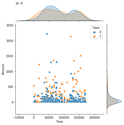
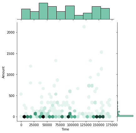
No noticable item to separate two classes only with Amount or Time. Unlike my expectation, the typical amount of fraud is very little.

Select features

We will select features which have high correlation with Class. While selecting features, other features with too high correlation with the selected feature will be dropped.

# sort features according to correlation with class 
sorted_features = df.corr().Class.abs().sort_values(ascending=False).drop('Class').index.to_numpy()

# features to drop
to_drop = set()

# add features to drop due to high correlation with another
for x in sorted_features:
    
    if x in to_drop:
        continue
    
    for y in sorted_features:
        
        if y in to_drop:
            continue
        elif x==y:
            continue
        else:
            val = df[x].corr(df[y])
            if val>0.85:
                to_drop.add(y)
print('Features to drop:',to_drop)

Features to drop: {'V12', 'V7', 'V16', 'V18', 'V3'}

# Select highly correlated features again
sorted_features = df.corr().Class.abs().sort_values(ascending=False).drop('Class').drop(list(to_drop))

print('Feature correlation with Class:\n', sorted_features)

Feature correlation with Class:
 V14       0.720942
V4        0.694075
V11       0.646819
V10       0.605722
V9        0.522540
V17       0.516138
V2        0.461733
V6        0.428790
V1        0.404820
V5        0.322045
V19       0.248267
V20       0.219867
V27       0.106493
V22       0.105856
V15       0.090137
V28       0.087062
V24       0.086127
Amount    0.085669
V21       0.079010
V8        0.073927
V23       0.065870
V13       0.038041
V25       0.031948
V26       0.028809
Time      0.026600
Name: Class, dtype: float64

# Dataframe for train and test

# Select 5 features for now, to check distribution
selected_features = sorted_features.iloc[:5]
train = df[selected_features.index.tolist()+['Class']]

# Visualize correlations and distributions
sns.pairplot(train, hue="Class")
plt.show()

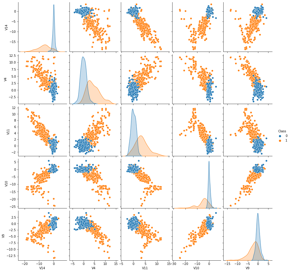
• From this pair plot, we can see that those selected features have high classification power.
• Also, each feature separates two classes with a single straight boundary. Logistic regression will perform well here.
• I noticed that the features are not scaled. Let’s do it.

Feature scaling

scaler = StandardScaler()

# fit with training set
scaler.fit(df.drop('Class',axis=1))

# transform all sets
df[df.columns[:-1]] = scaler.transform(df.drop('Class',axis=1))
df_dev[df_dev.columns[:-1]] = scaler.transform(df_dev.drop('Class',axis=1))
df_test[df_test.columns[:-1]] = scaler.transform(df_test.drop('Class',axis=1))

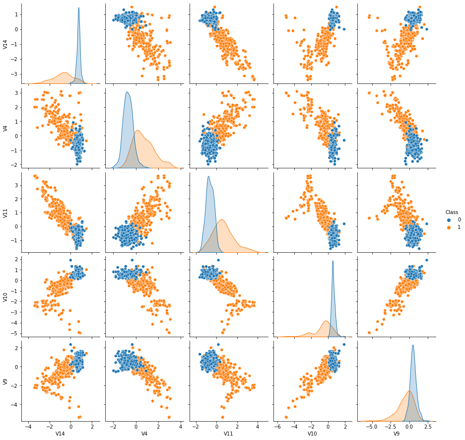
# Confirm transformation result
train = df[selected_features.index.tolist()+['Class']]

sns.pairplot(train, hue="Class")
plt.show()

Train

Let’s train and plot learning curve. For the cost function, I’ll use cross entropy.

def learning_curve_wrapper(X,y):
    
    n_samples = X.shape[0]
    cv = ShuffleSplit(n_splits=10, test_size=0.3, random_state=0)

    model = LogisticRegression()
    #scorer = make_scorer(recall_score, greater_is_better=True)
    scorer = make_scorer(log_loss, greater_is_better=False)

    title = "Learning Curves"

    plot_learning_curve(model, title, X, y, scoring=scorer, train_sizes=np.linspace(.1, 1.0, 20))


    plt.show()
    
    return model

fsize(12,6)    
model = learning_curve_wrapper(train[train.columns[:-1]], train.Class)

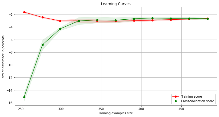
Both of training and validation scores saturated at the similar score. No sign of overfit.

Hypermarameter tuning

Hyper parameters can be

• Number of selected features
• Regularization parameters.

Here, I’ll try with l1 and l2 regularization with “liblinear” obtimization algorithm because it is a good choice for small dataset.

# loop over scoring metric
model_var = []
imodel = 0
#for scoring in ['recall','accuracy','precision', 'f1']:
    
# loop over number of features
for num_features in range(1,20): 

    selected_features = sorted_features.iloc[:num_features]

    train = df[selected_features.index.tolist()+['Class']]
    dev = df_dev[selected_features.index.tolist()+['Class']]

    X_train = train[train.columns[:-1]]
    y_train = train.Class
    X_dev = dev[dev.columns[:-1]]
    y_dev = dev.Class        

    # logistic regression with L2 regularization
    # obtimization is liblinear
    model = LogisticRegression(solver='liblinear')

    penalty= ['l1','l2']

    # inverse of regularization strength
    # smaller values specify stronger regularization
    C = [100, 30, 10, 3.0, 1.0, 0.3, 0.1, 0.03, 0.01]

    # dictionary of hyperparameters
    distributions = dict(penalty=penalty, C=C)

    # grid search
    clf = GridSearchCV(model, distributions, scoring='neg_log_loss', cv=5)

    search = clf.fit(X_train, y_train)

    # best hyperparameter dict
    bp = search.best_params_

    # test score with vaildation set
    model = LogisticRegression(solver='liblinear', penalty=bp['penalty'], C=bp['C'])       
    model.fit(X_train, y_train)
    y_pred = model.predict(X_dev)
    y_proba = model.predict_proba(X_dev)
    y_proba = y_proba[:,1]

    rc = recall_score(y_dev,y_pred)
    ac = accuracy_score(y_dev,y_pred)
    pr = precision_score(y_dev,y_pred) 
    f1 = f1_score(y_dev,y_pred)

    
    coefs = pd.Series(model.coef_.flatten(), index = selected_features.index.tolist())
    
    model_var.append([imodel,model,coefs,num_features])#, y_pred,y_proba])


    print(imodel, num_features, bp, '\t', round(rc, 3),round(ac, 3),round(pr, 3),round(f1, 3) )

    imodel+=1

0 1 {'C': 30, 'penalty': 'l2'} 	 0.947 0.961 0.973 0.96
1 2 {'C': 10, 'penalty': 'l2'} 	 0.934 0.934 0.934 0.934
2 3 {'C': 3.0, 'penalty': 'l2'} 	 0.934 0.941 0.947 0.94
3 4 {'C': 3.0, 'penalty': 'l2'} 	 0.934 0.947 0.959 0.947
4 5 {'C': 3.0, 'penalty': 'l2'} 	 0.947 0.954 0.96 0.954
5 6 {'C': 3.0, 'penalty': 'l2'} 	 0.934 0.947 0.959 0.947
6 7 {'C': 3.0, 'penalty': 'l2'} 	 0.934 0.954 0.973 0.953
7 8 {'C': 3.0, 'penalty': 'l2'} 	 0.947 0.954 0.96 0.954
8 9 {'C': 3.0, 'penalty': 'l2'} 	 0.947 0.961 0.973 0.96
9 10 {'C': 3.0, 'penalty': 'l2'} 	 0.947 0.961 0.973 0.96
10 11 {'C': 3.0, 'penalty': 'l2'} 	 0.947 0.961 0.973 0.96
11 12 {'C': 3.0, 'penalty': 'l2'} 	 0.947 0.961 0.973 0.96
12 13 {'C': 1.0, 'penalty': 'l1'} 	 0.947 0.961 0.973 0.96
13 14 {'C': 1.0, 'penalty': 'l1'} 	 0.947 0.954 0.96 0.954
14 15 {'C': 1.0, 'penalty': 'l1'} 	 0.947 0.954 0.96 0.954
15 16 {'C': 1.0, 'penalty': 'l1'} 	 0.947 0.947 0.947 0.947
16 17 {'C': 1.0, 'penalty': 'l1'} 	 0.947 0.947 0.947 0.947
17 18 {'C': 1.0, 'penalty': 'l2'} 	 0.947 0.961 0.973 0.96
18 19 {'C': 1.0, 'penalty': 'l2'} 	 0.934 0.954 0.973 0.953

Overall, performances are similar. Best Model 5 has slightly better performance, but it changes whenever I run the code (I don’t know if I can fix random state of GridSearchCV). For closer look, let’s plot feature coefficient together for first few cases.

# Plot features with high coefficient (leading features)
fsize(12,30,True)
for i in range(0,14):
    
    plt.subplot(7,2,i+1)
    
    _, model, coefs, num_features = model_var[i]
    
    #coefs = pd.concat([coefs.sort_values().head(7),
     #                coefs.sort_values().tail(8)])
    coefs.plot.barh()
    plt.xlabel('Coefficient')
    ax = plt.title("Coefficients")

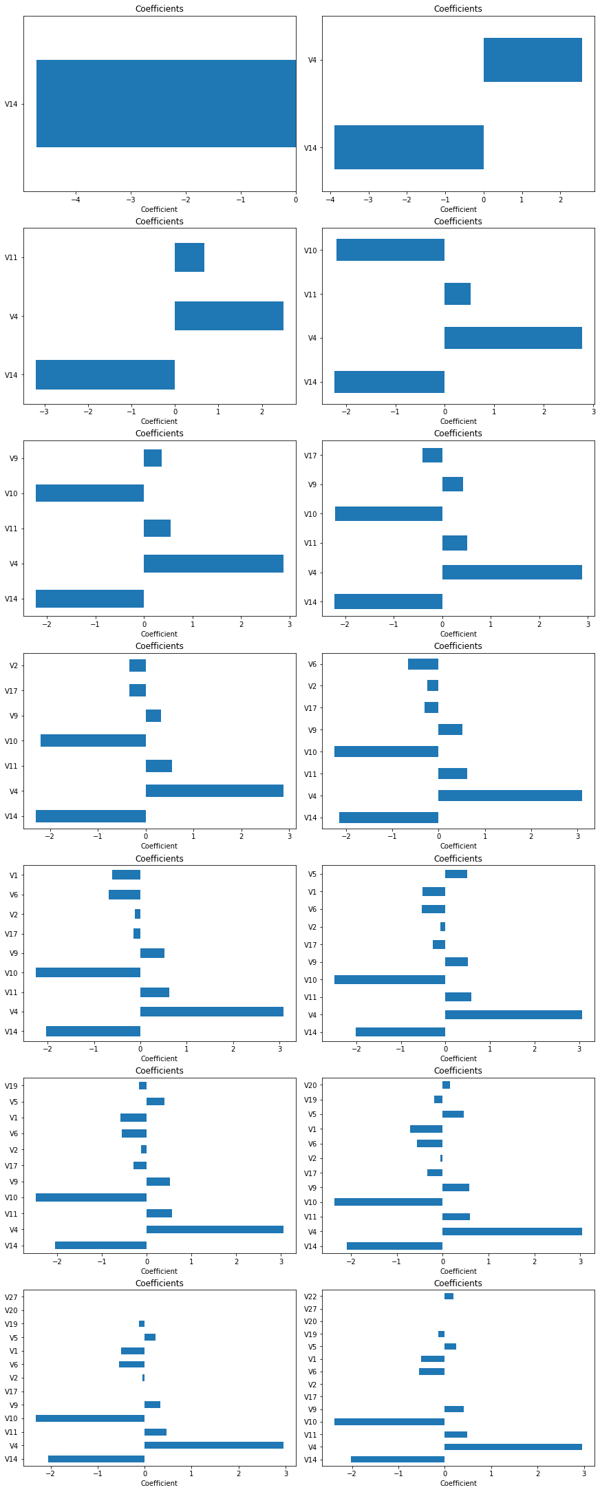
While coefficients of the first four leading components look quite consistent, 5th component was not stable. Also, V1 and V5 components seem to contribute quite a lot consistently. Let’s try include them along with the first four component, and see if it improves this model.

train = df[['V14','V4','V11','V10','V1','V5','Class']]
dev = df_dev[['V14','V4','V11','V10','V1','V5','Class']]

X_train = train[train.columns[:-1]]
y_train = train.Class
X_dev = dev[dev.columns[:-1]]
y_dev = dev.Class        

# logistic regression with L2 regularization
# obtimization is liblinear
model = LogisticRegression(solver='liblinear')

penalty= ['l1','l2']

# inverse of regularization strength
# smaller values specify stronger regularization
C = [100, 30, 10, 3.0, 1.0, 0.3, 0.1, 0.03, 0.01]

# dictionary of hyperparameters
distributions = dict(penalty=penalty, C=C)

# grid search
clf = GridSearchCV(model, distributions, scoring='neg_log_loss', cv=5)

search = clf.fit(X_train, y_train)

# best hyperparameter dict
bp = search.best_params_

# test score with vaildation set
model = LogisticRegression(solver='liblinear', penalty=bp['penalty'], C=bp['C'])       
model.fit(X_train, y_train)
y_pred = model.predict(X_dev)
y_proba = model.predict_proba(X_dev)
y_proba = y_proba[:,1]

rc = recall_score(y_dev,y_pred)
ac = accuracy_score(y_dev,y_pred)
pr = precision_score(y_dev,y_pred) 
f1 = f1_score(y_dev,y_pred)


coefs = pd.Series(model.coef_.flatten(), index = ['V14','V4','V11','V10','V1','V5'])

print(bp, '\t', round(rc, 3),round(ac, 3),round(pr, 3),round(f1, 3) )

{'C': 3.0, 'penalty': 'l2'} 	 0.934 0.947 0.959 0.947

No, it didn’t improve.

So, for our final model, let’s include only the first 4 components, which were leading components consistently. This model number is 3.

Test and Results

# get a final model
_, model, coefs, num_features = model_var[3]

selected_features = sorted_features.iloc[:num_features]

X_test = df[selected_features.index]
y_test = df.Class

# get prediction
y_pred = model.predict(X_test)
y_proba = model.predict_proba(X_test)
y_proba = y_proba[:,1]

# print scores
rc = recall_score(y_test,y_pred)
ac = accuracy_score(y_test,y_pred)
pr = precision_score(y_test,y_pred) 
f1 = f1_score(y_test,y_pred)

print('Scores:',round(rc, 3),round(ac, 3),round(pr, 3),round(f1, 3) )
print(selected_features, model.coef_, model.intercept_)

print(confusion_matrix(y_test, y_pred))

Scores: 0.871 0.925 0.978 0.921
V14    0.720942
V4     0.694075
V11    0.646819
V10    0.605722
Name: Class, dtype: float64 [[-2.23133532  2.77847589  0.519276   -2.19161554]] [2.68467681]
[[296   6]
 [ 39 263]]

V14, V4, and V10 played the most significant contribution. This model gave high recall score, 0.90, while giving very high precision, 0.98.

fsize(16,10)

test = X_test.copy()
test['Class'] = y_test


plt.subplot(2,2,1)
plt.scatter(X_test.V14, y_test, alpha=0.2)
plt.xlabel('V14')
plt.ylabel('Class')


plt.subplot(2,2,2)
plt.scatter(X_test.V4, y_test, alpha=0.2)
plt.xlabel('V4')
plt.ylabel('Class')


plt.subplot(2,2,3)

test['pred']= y_pred

X = test[(test.Class==0)&(test.pred==0)]
plt.scatter(X.V14, X.V4, color='tab:blue', alpha=0.1, label='Normal')

X = test[(test.Class==0)&(test.pred==1)]
plt.scatter(X.V14, X.V4, color='tab:blue', marker='x', label='Normal, predicted fraud')

X = test[(test.Class==1)&(test.pred==1)]
plt.scatter(X.V14, X.V4, color='tab:orange', alpha=0.1, label='Fraud')

X = test[(test.Class==1)&(test.pred==0)]
plt.scatter(X.V14, X.V4, color='tab:orange', marker='x', label='Fraud, predicted normal')

plt.xlabel('V14')
plt.ylabel('V4')
plt.legend()


plt.subplot(2,2,4)

X = test[(test.Class==0)&(test.pred==0)]
plt.scatter(X.V14, X.V10, color='tab:blue', alpha=0.1, label='Normal')

X = test[(test.Class==0)&(test.pred==1)]
plt.scatter(X.V14, X.V10, color='tab:blue', marker='x', label='Normal, predicted fraud')

X = test[(test.Class==1)&(test.pred==1)]
plt.scatter(X.V14, X.V10, color='tab:orange', alpha=0.1, label='Fraud')

X = test[(test.Class==1)&(test.pred==0)]
plt.scatter(X.V14, X.V10, color='tab:orange', marker='x', label='Fraud, predicted normal')

plt.xlabel('V14')
plt.ylabel('V10')
plt.legend()

<matplotlib.legend.Legend at 0x7fea801a6fa0>

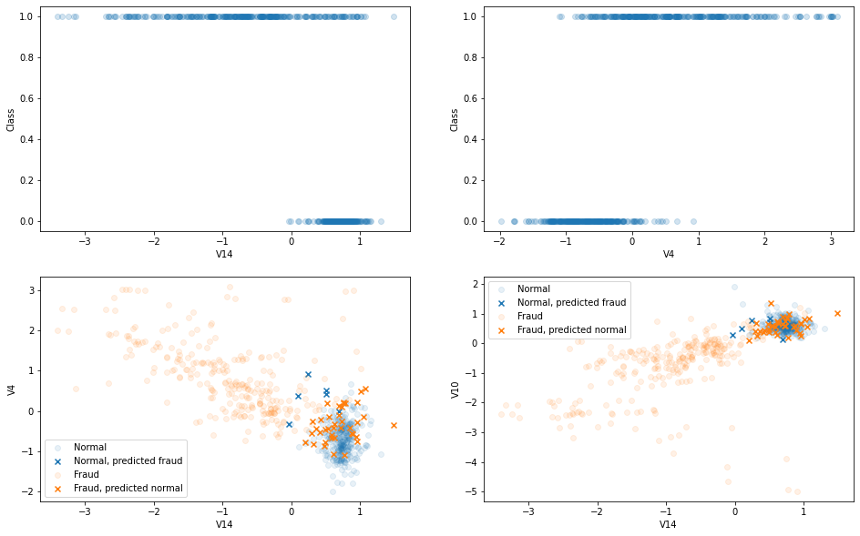
Those plots visualize class overlapping regions.

# plot probabilities
fsize(8,6)
X = test[test.Class==0].drop(['Class','pred'],axis=1)
ax =plt.hist(model.predict_proba(X)[:,1], bins=30, range=(0,1), label='Normal', alpha=0.4)

X = test[test.Class==1].drop(['Class','pred'],axis=1)
ax = plt.hist(model.predict_proba(X)[:,1], bins=30, range=(0,1), label='Fraud', alpha=0.4)

plt.xlabel('Predicted probability of Fraud')
plt.legend()

<matplotlib.legend.Legend at 0x7fea80239bb0>

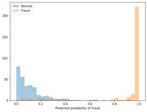
While fraud events have a peak at predicted probability around 1, the predicted probability of normal transactions is more even out. This model is more strict for fraud.

# Plot ROC curve
fsize(8,6)
fpr, tpr, thr = roc_curve(y_test, y_proba)

plt.plot(fpr, tpr, color='red', label='ROC')
plt.plot([0, 1], [0, 1], color='green', linestyle='--')
plt.xlabel('False Positive Rate')
plt.ylabel('True Positive Rate')
plt.title('Receiver Operating Characteristic Curve')
plt.legend()
plt.show()    

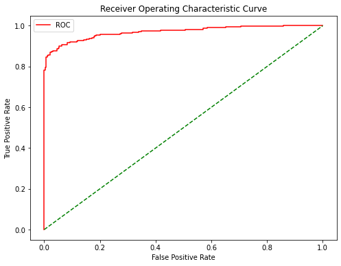
Around TPR=0.8, false alarm rate start to increase rapidly. We might invent a two steps detection system, such as record anything over threshold of TPR=0.8, then immediately stop transaction following a model optimized for the high precision.