Credit Card Fraud Detection with K-Nearest Neighbors
Intro
We will build a logistic regression model using PCA transformed data. Dataset: data/creditcard.csv source: Kaggle Previously, I built this model with Logistig regression. Let’t compare performance with kNN.
Here, I’ll skip EDA and use the same feature engineering as I’d done for Logistic regressions.
Import packages
from freq_utils import fsize # freq_utils.py is my custom file

import numpy as np
import pandas as pd
import matplotlib.pyplot as plt

from sklearn.neighbors import KNeighborsClassifier
from sklearn.model_selection import train_test_split
from sklearn.metrics import confusion_matrix
from sklearn.metrics import accuracy_score, precision_score, recall_score, f1_score, roc_auc_score
from sklearn.preprocessing import StandardScaler
Read dataset
df_read = pd.read_csv("data/creditcard.csv")

# drop duplication
df_read.drop_duplicates(inplace=True)
Undersampling and Train Test Split
To make kNN works fairly, class should be sampled in valance. I’ll balance the number of samples by undersampling since we have enough data.
Then split train and test sets.
# Split datasets separatively for each class
normal = df_read[df_read.Class==0]
fraud = df_read[df_read.Class==1]

# In kNN, there's no model building thing. I think important thing is to determine proper k using dev set.
# To have good amount of data to determin k using dev set, I'll give more data to dev set than usual.
normal0, normal2 =  train_test_split(normal, test_size = 0.2, random_state=1)
normal0, normal1 =  train_test_split(normal0, test_size = 0.5, random_state=2)

fraud0, fraud2 =  train_test_split(fraud, test_size = 0.2, random_state=3)
fraud0, fraud1 =  train_test_split(fraud0, test_size = 0.5, random_state=4)

# Undersampling for training and dev sets
df = pd.concat([fraud0,normal0.sample(len(fraud0))])
df_dev = pd.concat([fraud1,normal1.sample(len(fraud1))])

# Make a test sample realistic, i.e. 0.172% of transactions are fraud
df_test = pd.concat([fraud2, normal2])
Feature engineering
Feature scaling
scaler = StandardScaler()

# fit with training set
scaler.fit(df.drop('Class',axis=1))

# transform all sets
df[df.columns[:-1]] = scaler.transform(df.drop('Class',axis=1))
df_dev[df_dev.columns[:-1]] = scaler.transform(df_dev.drop('Class',axis=1))
df_test[df_test.columns[:-1]] = scaler.transform(df_test.drop('Class',axis=1))
Feature selection
See logistic regression.
selected_features = ['V14','V4','V11','V10'] # determined from logistic regression project

X_train = df[selected_features]
X_dev   = df_dev[selected_features]
X_test  = df_test[selected_features]

y_train = df.Class
y_dev = df_dev.Class
y_test = df_test.Class
Hyperparameter tuning
Nothing special for training. It is simple. Let’s jump to hyperparameter tuning.
# list to save scores of each k
scores = []

for k in range(1,100): # I should find how the KNeighborsClassifier solves tie for even k

    # pass training data info
    model = KNeighborsClassifier(n_neighbors = k)
    model.fit(X_train, y_train)


    # get prediction of dev set
    y_pred = model.predict(X_dev)

    # print scores
    rc = recall_score(y_dev,y_pred)
    ac = accuracy_score(y_dev,y_pred)
    pr = precision_score(y_dev,y_pred)
    f1 = f1_score(y_dev,y_pred)
    ra = roc_auc_score(y_dev,y_pred)

    # append scores
    scores.append([k, rc,ac,pr,f1,ra, model])

    print('k=',k, '\t', round(rc, 3),round(ac, 3),round(pr, 3),round(f1, 3),round(ra, 3) )
k= 1 	 0.905 0.899 0.895 0.9 0.899
k= 2 	 0.878 0.923 0.965 0.92 0.923
k= 3 	 0.926 0.939 0.951 0.938 0.939
k= 4 	 0.894 0.944 0.994 0.942 0.944
k= 5 	 0.905 0.939 0.972 0.937 0.939
k= 6 	 0.878 0.934 0.988 0.93 0.934
k= 7 	 0.894 0.929 0.96 0.926 0.929
k= 8 	 0.878 0.934 0.988 0.93 0.934
k= 9 	 0.894 0.934 0.971 0.931 0.934
k= 10 	 0.889 0.934 0.977 0.931 0.934
k= 11 	 0.889 0.926 0.96 0.923 0.926
k= 12 	 0.884 0.931 0.977 0.928 0.931
k= 13 	 0.889 0.929 0.966 0.926 0.929
k= 14 	 0.889 0.931 0.971 0.928 0.931
k= 15 	 0.894 0.931 0.966 0.929 0.931
k= 16 	 0.884 0.931 0.977 0.928 0.931
k= 17 	 0.884 0.923 0.96 0.92 0.923
k= 18 	 0.884 0.926 0.965 0.923 0.926
k= 19 	 0.884 0.923 0.96 0.92 0.923
k= 20 	 0.884 0.931 0.977 0.928 0.931
k= 21 	 0.884 0.931 0.977 0.928 0.931
k= 22 	 0.884 0.934 0.982 0.93 0.934
k= 23 	 0.884 0.931 0.977 0.928 0.931
k= 24 	 0.884 0.937 0.988 0.933 0.937
k= 25 	 0.884 0.937 0.988 0.933 0.937
k= 26 	 0.878 0.934 0.988 0.93 0.934
k= 27 	 0.884 0.937 0.988 0.933 0.937
k= 28 	 0.884 0.937 0.988 0.933 0.937
k= 29 	 0.884 0.937 0.988 0.933 0.937
k= 30 	 0.878 0.934 0.988 0.93 0.934
k= 31 	 0.884 0.937 0.988 0.933 0.937
k= 32 	 0.878 0.937 0.994 0.933 0.937
k= 33 	 0.884 0.937 0.988 0.933 0.937
k= 34 	 0.884 0.939 0.994 0.936 0.939
k= 35 	 0.884 0.939 0.994 0.936 0.939
k= 36 	 0.878 0.937 0.994 0.933 0.937
k= 37 	 0.878 0.937 0.994 0.933 0.937
k= 38 	 0.878 0.937 0.994 0.933 0.937
k= 39 	 0.878 0.937 0.994 0.933 0.937
k= 40 	 0.878 0.937 0.994 0.933 0.937
k= 41 	 0.878 0.937 0.994 0.933 0.937
k= 42 	 0.878 0.937 0.994 0.933 0.937
k= 43 	 0.878 0.937 0.994 0.933 0.937
k= 44 	 0.878 0.939 1.0 0.935 0.939
k= 45 	 0.878 0.939 1.0 0.935 0.939
k= 46 	 0.878 0.939 1.0 0.935 0.939
k= 47 	 0.878 0.939 1.0 0.935 0.939
k= 48 	 0.873 0.937 1.0 0.932 0.937
k= 49 	 0.878 0.939 1.0 0.935 0.939
k= 50 	 0.873 0.937 1.0 0.932 0.937
k= 51 	 0.873 0.937 1.0 0.932 0.937
k= 52 	 0.873 0.937 1.0 0.932 0.937
k= 53 	 0.873 0.937 1.0 0.932 0.937
k= 54 	 0.873 0.937 1.0 0.932 0.937
k= 55 	 0.873 0.937 1.0 0.932 0.937
k= 56 	 0.873 0.937 1.0 0.932 0.937
k= 57 	 0.873 0.937 1.0 0.932 0.937
k= 58 	 0.873 0.937 1.0 0.932 0.937
k= 59 	 0.873 0.937 1.0 0.932 0.937
k= 60 	 0.868 0.934 1.0 0.929 0.934
k= 61 	 0.868 0.934 1.0 0.929 0.934
k= 62 	 0.868 0.934 1.0 0.929 0.934
k= 63 	 0.868 0.934 1.0 0.929 0.934
k= 64 	 0.868 0.934 1.0 0.929 0.934
k= 65 	 0.868 0.934 1.0 0.929 0.934
k= 66 	 0.868 0.934 1.0 0.929 0.934
k= 67 	 0.868 0.934 1.0 0.929 0.934
k= 68 	 0.868 0.934 1.0 0.929 0.934
k= 69 	 0.868 0.934 1.0 0.929 0.934
k= 70 	 0.868 0.934 1.0 0.929 0.934
k= 71 	 0.868 0.934 1.0 0.929 0.934
k= 72 	 0.868 0.934 1.0 0.929 0.934
k= 73 	 0.868 0.934 1.0 0.929 0.934
k= 74 	 0.868 0.934 1.0 0.929 0.934
k= 75 	 0.868 0.934 1.0 0.929 0.934
k= 76 	 0.868 0.934 1.0 0.929 0.934
k= 77 	 0.868 0.934 1.0 0.929 0.934
k= 78 	 0.868 0.934 1.0 0.929 0.934
k= 79 	 0.868 0.934 1.0 0.929 0.934
k= 80 	 0.868 0.934 1.0 0.929 0.934
k= 81 	 0.868 0.934 1.0 0.929 0.934
k= 82 	 0.868 0.934 1.0 0.929 0.934
k= 83 	 0.868 0.934 1.0 0.929 0.934
k= 84 	 0.868 0.934 1.0 0.929 0.934
k= 85 	 0.868 0.934 1.0 0.929 0.934
k= 86 	 0.868 0.934 1.0 0.929 0.934
k= 87 	 0.868 0.934 1.0 0.929 0.934
k= 88 	 0.868 0.934 1.0 0.929 0.934
k= 89 	 0.868 0.934 1.0 0.929 0.934
k= 90 	 0.868 0.934 1.0 0.929 0.934
k= 91 	 0.868 0.934 1.0 0.929 0.934
k= 92 	 0.868 0.934 1.0 0.929 0.934
k= 93 	 0.868 0.934 1.0 0.929 0.934
k= 94 	 0.868 0.934 1.0 0.929 0.934
k= 95 	 0.868 0.934 1.0 0.929 0.934
k= 96 	 0.868 0.934 1.0 0.929 0.934
k= 97 	 0.868 0.934 1.0 0.929 0.934
k= 98 	 0.868 0.934 1.0 0.929 0.934
k= 99 	 0.868 0.934 1.0 0.929 0.934
# Plot dev sert scores
fsize(12,8)

# reconstruct tuning parameters lists
k = [x[0] for x in scores]
rc = [x[1] for x in scores]
ac = [x[2] for x in scores]
pr = [x[3] for x in scores]
f1 = [x[4] for x in scores]
ra = [x[5] for x in scores]

# plot
plt.plot(k,rc,label='Recall')
plt.plot(k,ac,label='Accuracy')
plt.plot(k,pr,label='Precision')
plt.plot(k,f1,label='F1 score')
plt.plot(k,ra,label='ROC AUC')
plt.legend()
plt.xlabel('k')
plt.ylabel('Score')
plt.title('Scores for different number of neighbors (k)')
plt.grid()
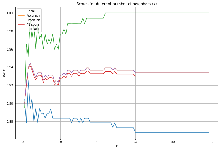
I’ll choose k=27 because it gave relatively good recall, F1, AUC scores, while k itself is not too small, having potential to overfit.
Test and Results
# final model: k=9
model = scores[9][6]

# get prediction of test set
y_pred = model.predict(X_test)

# print scores
print('Accuracy:',accuracy_score(y_test, y_pred))
print('Precision:',precision_score(y_test, y_pred))
print('Recall:',recall_score(y_test, y_pred))
print('F1:',f1_score(y_test, y_pred))
print('ROC AUC:',roc_auc_score(y_test, y_pred))
Accuracy: 0.9814612483699292
Precision: 0.07390917186108638
Recall: 0.8736842105263158
F1: 0.13628899835796388
ROC AUC: 0.9276630969490945
Recall is great, but precision is terrible. High accuracy is meaningless because of highly imbalanced dataset. The result is worse than the logistic regression model we built previously.
# plot distributions for leading two features
fsize(6,6)

test = X_test.copy()

test['pred']= y_pred
test['Class'] = y_test

X = test[(test.Class==0)&(test.pred==0)]
plt.scatter(X.V14, X.V4, color='tab:blue', alpha=0.1, label='Normal')

X = test[(test.Class==0)&(test.pred==1)]
plt.scatter(X.V14, X.V4, color='tab:blue', marker='x', label='Normal, predicted fraud')

X = test[(test.Class==1)&(test.pred==1)]
plt.scatter(X.V14, X.V4, color='tab:orange', alpha=0.1, label='Fraud')

X = test[(test.Class==1)&(test.pred==0)]
plt.scatter(X.V14, X.V4, color='tab:orange', marker='x', label='Fraud, predicted normal')

plt.xlabel('V14')
plt.ylabel('V4')
plt.legend(loc=3)
<matplotlib.legend.Legend at 0x7fccd8f387f0>
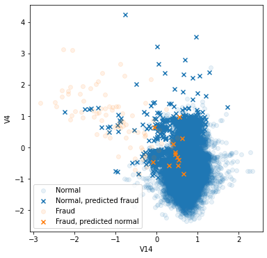
We didn’t miss too much fraud transaction, as also seen from the high recall score. However, we marked too much of normal transaction as fraud. Compared to logistic regression, here’s what I guess.
- From the plot above, the normal events are spread over large area whereas fraud events are not. Fraud events have more density, so it has advantage to be selected as “the nearest neighbor”.
Conclusion - comparison to logistic regression
Overall, the performance of logistic regression was better than kNN in this project. I can list two main reasons which explain why.
- Fraud events are more dense in the n (number of used features) dimension space. That made kNN to select fraud events more in the thick gray area.
- Two classes are separated with a linear decision boundary. In this case, logistic regression works well.
Leave a comment